Baseline#
Before we dive into some models, let’s define the heuristic that must be beaten. It is not just the case for RecSys the problem, but in all ML projects you better start with a definition of baseline to understand the efficiency of your model. Sometimes it is the case that some heuristics-based algorithm will do the work and it is ok – the goal is your users and business value and having an exceptional ML model is not the goal at all.
There are various ways to generate baseline recommendations. One of them is to recommend popular items based on some metrics like rating, and counters (watch times, number of purchases, clicks, etc.). Also, we can use grouping based on user segments to make more accurate and relevant recommendations (to some extent, of course :)). Here, we will use mean rating as a proxy for popularity and recommendations
In this chapter, I will walk through baseline recommender using MovieLens Data For convenience, I uploaded it to Google Drive for centralized access for anyone. Below, there are the URLs of the main datasets that will be used for the baseline recommender.
0. Configuration#
# links to shared data MovieLens
RATINGS_SMALL_URL = 'http://drive.google.com/file/d/1BlZfCLLs5A13tbNSJZ1GPkHLWQOnPlE4/view?usp=share_link'
MOVIES_METADATA_URL = 'http://drive.google.com/file/d/19g6-apYbZb5D-wRj4L7aYKhxS-fDM4Fb/view?usp=share_link'
1. Modules and functions#
Now, let’s import some libraries
# just to make it available to download w/o SSL verification
import ssl
ssl._create_default_https_context = ssl._create_unverified_context

import numpy as np
import pandas as pd
import matplotlib.pyplot as plt

from itertools import islice, cycle, product

import warnings
warnings.filterwarnings('ignore')
pd.set_option('display.float_format', lambda x: '%.2f' % x)
and define 2 useful functinons 1) read_csv_from_gdrive() to get data from provided url of a file
def read_csv_from_gdrive(url):
    """
    gets csv data from a given url (taken from file -> share -> copy link)
    :url: example https://drive.google.com/file/d/1BlZfCLLs5A13tbNSJZ1GPkHLWQOnPlE4/view?usp=share_link
    """
    file_id = url.split('/')[-2]
    file_path = 'https://drive.google.com/uc?export=download&id=' + file_id
    data = pd.read_csv(file_path)

    return data
2nd one is compute_popularity() which calculates mean rating, sorts and returns top K required items
def compute_popularity(df: pd.DataFrame, item_id: str, max_candidates: int):
    """
    calculates mean rating to define popular titles
    """
    popular_titles = df.groupby(item_id).agg({'rating': np.mean})\
                     .sort_values(['rating'], ascending=False).head(max_candidates).index.values

    return popular_titles
2. Data#
2.1 Load and Describe#
Here, we will use two datasets:
interactions – refers to
RATINGS_SMALL_URLwhere we have userId, movieId, timestamp and rating (our so-called target)movies_metadata – refers to
MOVIES_METADATA_URLwhere we have data all about movies - overview, genres etc.
# interactions data
interactions = read_csv_from_gdrive(RATINGS_SMALL_URL)
interactions.head()
| userId | movieId | rating | timestamp | |
|---|---|---|---|---|
| 0 | 1 | 31 | 2.50 | 1260759144 |
| 1 | 1 | 1029 | 3.00 | 1260759179 |
| 2 | 1 | 1061 | 3.00 | 1260759182 |
| 3 | 1 | 1129 | 2.00 | 1260759185 |
| 4 | 1 | 1172 | 4.00 | 1260759205 |
Let’s get some statistics and look at ratings’ distribution
interactions.describe()
| userId | movieId | rating | timestamp | |
|---|---|---|---|---|
| count | 100004.00 | 100004.00 | 100004.00 | 100004.00 |
| mean | 347.01 | 12548.66 | 3.54 | 1129639086.94 |
| std | 195.16 | 26369.20 | 1.06 | 191685826.03 |
| min | 1.00 | 1.00 | 0.50 | 789652009.00 |
| 25% | 182.00 | 1028.00 | 3.00 | 965847824.00 |
| 50% | 367.00 | 2406.50 | 4.00 | 1110421822.00 |
| 75% | 520.00 | 5418.00 | 4.00 | 1296192495.50 |
| max | 671.00 | 163949.00 | 5.00 | 1476640644.00 |
plt.style.use('ggplot')
interactions['rating'].hist();
plt.title('Ratings Distribtion');
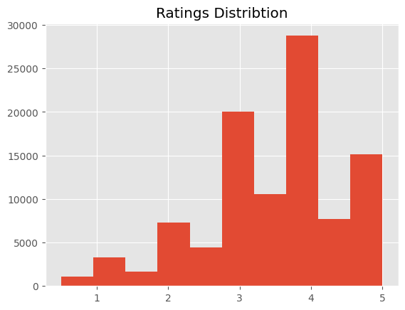
We see that in most cases we have a 4 or 5 rating - the right tail is fatter. Now, let’s move on to movies metadata
# information about films etc
movies_metadata = read_csv_from_gdrive(MOVIES_METADATA_URL)
Which columns / info we have and their types - namings are pretty straightforward
movies_metadata.info()
<class 'pandas.core.frame.DataFrame'>
RangeIndex: 45466 entries, 0 to 45465
Data columns (total 24 columns):
 #   Column                 Non-Null Count  Dtype
---  ------                 --------------  -----
 0   adult                  45466 non-null  object
 1   belongs_to_collection  4494 non-null   object
 2   budget                 45466 non-null  object
 3   genres                 45466 non-null  object
 4   homepage               7782 non-null   object
 5   id                     45466 non-null  object
 6   imdb_id                45449 non-null  object
 7   original_language      45455 non-null  object
 8   original_title         45466 non-null  object
 9   overview               44512 non-null  object
 10  popularity             45461 non-null  object
 11  poster_path            45080 non-null  object
 12  production_companies   45463 non-null  object
 13  production_countries   45463 non-null  object
 14  release_date           45379 non-null  object
 15  revenue                45460 non-null  float64
 16  runtime                45203 non-null  float64
 17  spoken_languages       45460 non-null  object
 18  status                 45379 non-null  object
 19  tagline                20412 non-null  object
 20  title                  45460 non-null  object
 21  video                  45460 non-null  object
 22  vote_average           45460 non-null  float64
 23  vote_count             45460 non-null  float64
dtypes: float64(4), object(20)
memory usage: 8.3+ MB
2.2. Data Preparation#
Here, we will
preprocess column names;
set similar typing;
leave movies in
interactionsthat are present inmovies_metadata;create users dataset for recommendatinos;
movies name and movie mapper for convenience
First, we need to merge two dataframes and for that, it is necessary to make appropriate typing and column names for convenience. The relationship between both datasets is set by movie id.
# align data in both dataframes to merge
interactions['movieId'] = interactions['movieId'].astype(str)
movies_metadata.rename(columns = {'id': 'movieId'}, inplace = True)
# leave only those films that intersect with each other
interactions_filtered = interactions.loc[interactions['movieId'].isin(movies_metadata['movieId'])]
print(interactions.shape, interactions_filtered.shape)
(100004, 4) (44989, 4)
# create users input
users = interactions[['userId']].drop_duplicates().reset_index(drop = True)
# create mapper for movieId and title names
item_name_mapper = dict(zip(movies_metadata['movieId'], movies_metadata['original_title']))
3. Model#
Let’s define our baseline popularity recommender BaselineRecommender - top-rated titles based on average rating with a possibility to get by any group(s)
The pipeline will be similar to most python ML modules – it will have two methods in the end: fit() and recommend()
The logic of fit() as follow:
Initiate recommendation based on a median rating from all observations recomm_common;
Prepare a list of interacted items by users
If we set groups - we get recommendations i.e. calculate movie ratings by groups:
If we get NaN, we fill it with base recommendations
If we get less than the required number of candidates, we populate from base recommendations
The logic of recommend():
Return base recommendations if users data is not set;
In the case of category wise requirements – we get results of our fit
3.1. Fit#
First, we define how many candidates we want to get
MAX_CANDIDATES = 20
ITEM_COLUMN = 'movieId'
USER_COLUMN = 'userId'
Then, we extract top 20 movies by aggregating movies and averaging rating column across all users
base_recommendations = compute_popularity(interactions_filtered, ITEM_COLUMN, MAX_CANDIDATES)
base_recommendations
array(['74727', '128846', '702', '127728', '65216', '43267', '8675',
       '80717', '86817', '8699', '872', '27724', '26791', '876', '64278',
       '301', '59392', '3021', '3112', '1933'], dtype=object)
Thus, we got 20 films with the highest average rating Now, as we discussed earlier, in movie recommendations there is no need to recommend the same film which the user has already watched. Let’s implement it as well We get all interacted items for each user and save them in dictionary {‘userId’: [items list]}
known_items = interactions_filtered.groupby(USER_COLUMN)[ITEM_COLUMN].apply(list).to_dict()
print(f"Number of users with known items: {len(known_items)} \n")

# let's check it for one userId = 1
print(f"Example of known item ids for particaular user: {known_items[1]}")
Number of users with known items: 671

Example of known item ids for particaular user: ['1371', '1405', '2105', '2193', '2294', '2455']
Now we have all the necessary components: base recommendations without groups with the possibility to filter already watched items Also, if we want to get recommendations based on some user groups we can easily do the same with groupby() method and the same approach
# lets add artifical binary group to check BaselineRecommender
group = [np.random.random_integers(2) for x in range(len(users))]
users['group'] = group
Here we merge it to get groupwise recommendations
data = pd.merge(interactions_filtered, users, how='left', on = USER_COLUMN)
group_recommendations = data.groupby('group').apply(compute_popularity, ITEM_COLUMN, MAX_CANDIDATES)
group_recommendations.head()
group
1    [3580, 3575, 876, 5121, 1649, 4519, 4772, 3432...
2    [4688, 26797, 26578, 91690, 49280, 4201, 26422...
dtype: object
In the output, we have two rows with a list of film ids for each binary group
Next, we have to implement recommend() method which will use
3.2. Recommend#
Earlier, we discussed that we can take just the average/median, etc. of rating and use it as a popularity metric to use as recommendations. Thus, if we do not have groups to consider (a.k.a more granular estimation), then it means we give the same recommendations for all users i.e. base_recommendations
recs = list(islice(cycle([base_recommendations]), len(users['userId'])))
users['rekkos'] = recs
users.head()
| userId | group | rekkos | |
|---|---|---|---|
| 0 | 1 | 2 | [74727, 128846, 702, 127728, 65216, 43267, 867... |
| 1 | 2 | 1 | [74727, 128846, 702, 127728, 65216, 43267, 867... |
| 2 | 3 | 2 | [74727, 128846, 702, 127728, 65216, 43267, 867... |
| 3 | 4 | 2 | [74727, 128846, 702, 127728, 65216, 43267, 867... |
| 4 | 5 | 1 | [74727, 128846, 702, 127728, 65216, 43267, 867... |
And let’s have an example with groups we created earlier
group_recommendations = group_recommendations.reset_index()
group_rekkos = pd.merge(users, group_recommendations, how = 'left', on = 'group')
group_rekkos.rename(columns = {0: 'group_wise_rekkos'}, inplace = True)
group_rekkos.head()
| userId | group | rekkos | group_wise_rekkos | |
|---|---|---|---|---|
| 0 | 1 | 2 | [74727, 128846, 702, 127728, 65216, 43267, 867... | [4688, 26797, 26578, 91690, 49280, 4201, 26422... |
| 1 | 2 | 1 | [74727, 128846, 702, 127728, 65216, 43267, 867... | [3580, 3575, 876, 5121, 1649, 4519, 4772, 3432... |
| 2 | 3 | 2 | [74727, 128846, 702, 127728, 65216, 43267, 867... | [4688, 26797, 26578, 91690, 49280, 4201, 26422... |
| 3 | 4 | 2 | [74727, 128846, 702, 127728, 65216, 43267, 867... | [4688, 26797, 26578, 91690, 49280, 4201, 26422... |
| 4 | 5 | 1 | [74727, 128846, 702, 127728, 65216, 43267, 867... | [3580, 3575, 876, 5121, 1649, 4519, 4772, 3432... |
We got our groupwise recommendations from 3.1. part and just joined them by a group of users assigned to Further, we will prettify our code and wrap it into functions
3.3. Wrap everything into pretty functions#
3.3.1. Fit Part#
In this function, we need to support 4 main parameters
data – it is going to be pandas classic DataFrame;
item_col – the name of the item id column so we can apply it on any dataset;
groups – if we need groupwise recommendations;
max_candidates – the number of recommendations to return
Thus, our function will get a pandas data frame with necessary data, calculate popularity for a given type - groupwise or not and return ids
def fit(
    data: pd.DataFrame,
    item_col: str,
    groups: list = None,
    max_candidates: int = 20
    ):
    """
    function runs all pipeline to generate recommendations based on given group
    :data: dataframe of interactions
    :item_col: item column name
    :groups: optional, list of groups column names to get recommendations
    :max_candidates: number of recommendations to return
    """

    if groups is not None:
        recommendations = data.groupby(groups).apply(compute_popularity, item_col, max_candidates)
    else:
        recommendations = compute_popularity(data, item_col, max_candidates)

    return recommendations
# check base recommendations
fit(data, item_col=ITEM_COLUMN)
array(['74727', '128846', '702', '127728', '65216', '43267', '8675',
       '80717', '86817', '8699', '872', '27724', '26791', '876', '64278',
       '301', '59392', '3021', '3112', '1933'], dtype=object)
# check group-wise
fit(data, item_col=ITEM_COLUMN, groups=['group'])
group
1    [3580, 3575, 876, 5121, 1649, 4519, 4772, 3432...
2    [4688, 26797, 26578, 91690, 49280, 4201, 26422...
dtype: object
3.3.2. Recommend Part#
Here, we just use calculated recommendations from the above method fit()
def recommend(
    users: pd.DataFrame,
    recommendations: pd.DataFrame,
    groups: list = None,
    K: int = 10
    ):
    """
    recommends items for a given list of users
    :users: series / list of users to recommend
    :recommendations: output of fit() function
    :groups: optional, list of groups column names to get recommendations
    :K: number of items to recommend (not always we want to show dozens of items instantly)
    """
    if groups is not None:
        output = pd.merge(users, recommendations.reset_index(), how = 'left', on = 'group')

    else:
        output = users.copy(deep = True)
        recs = list(islice(cycle([recommendations]), len(users['userId'])))
        output['rekkos'] = recs

    return output
# check base recommendations
recs = fit(data, item_col=ITEM_COLUMN)
check_recs = recommend(users[['userId', 'group']], recs)
check_recs.head()
| userId | group | rekkos | |
|---|---|---|---|
| 0 | 1 | 2 | [74727, 128846, 702, 127728, 65216, 43267, 867... |
| 1 | 2 | 1 | [74727, 128846, 702, 127728, 65216, 43267, 867... |
| 2 | 3 | 2 | [74727, 128846, 702, 127728, 65216, 43267, 867... |
| 3 | 4 | 2 | [74727, 128846, 702, 127728, 65216, 43267, 867... |
| 4 | 5 | 1 | [74727, 128846, 702, 127728, 65216, 43267, 867... |
# check group-wise
recs = fit(data, item_col=ITEM_COLUMN, groups = ['group'])
check_recs = recommend(users[['userId', 'group']], recs, ['group'])
check_recs.head()
| userId | group | 0 | |
|---|---|---|---|
| 0 | 1 | 2 | [4688, 26797, 26578, 91690, 49280, 4201, 26422... |
| 1 | 2 | 1 | [3580, 3575, 876, 5121, 1649, 4519, 4772, 3432... |
| 2 | 3 | 2 | [4688, 26797, 26578, 91690, 49280, 4201, 26422... |
| 3 | 4 | 2 | [4688, 26797, 26578, 91690, 49280, 4201, 26422... |
| 4 | 5 | 1 | [3580, 3575, 876, 5121, 1649, 4519, 4772, 3432... |
Congrats! Your first basic recommender system is ready!! In the next section, we will dive into how to evaluate our model